Some models use an object class that handles one-dimensional heat conduction
through a number of layers of non-linear and phase-changing materials.
The object gets its data from the file material.sys
for all layer materials selected by the user.
The space discretisation uses the line method and the time integration a two-step implicit Runge-Kutta method.
The employed method is described by
Even Thorbergsen in his PhD thesis.
Each layer consists of a number of node intervals (a maximum of 50).
The node intervals may have a constant size or alternatively a varying size
where each consecutive interval is a fixed percentage of the previous.
The initial layer temperatures are specified as a linear distribution (with constant values a special case of this).
A layer can be inspected in the corresponding layer dialogue, displaying the distribution of
temperature, thermal conductivity, volumetric heat capacity and internal heat generation (source or sink).
Normally the heat conduction calculation is performed after the plant calculation has converged
and based on a linear interpolation between the temperatures at the start and end of the plant time step.
Therefore the accuracy is very much influenced by the plant time step.
Reduce this until the results are no more influenced by further reductions.
The plant time step is set by or .
The time step can be influenced by setting the minimum and maximum temperature change per time step
in the accuracy dialogue entered through the dialogue.
It is possible to do a simulation where the heat condition calculation is repeated from the start
for every iteration of the plant calculation, until this converges.
This will be an alternative to reducing the time step.
The total number of node intervals for a complete geometry is 500.
Increasing the number of node intervals is another way to achieve a higher accuracy.
The boundary conditions at the two opposite sides are set through boundary objects, each of which
may be inspected through the hosting component.
Through the menu command you get a report file for every component containing
a one-dimensional heat conduction object. The name of the file is the hosting component's name, while the type is H1D.
.
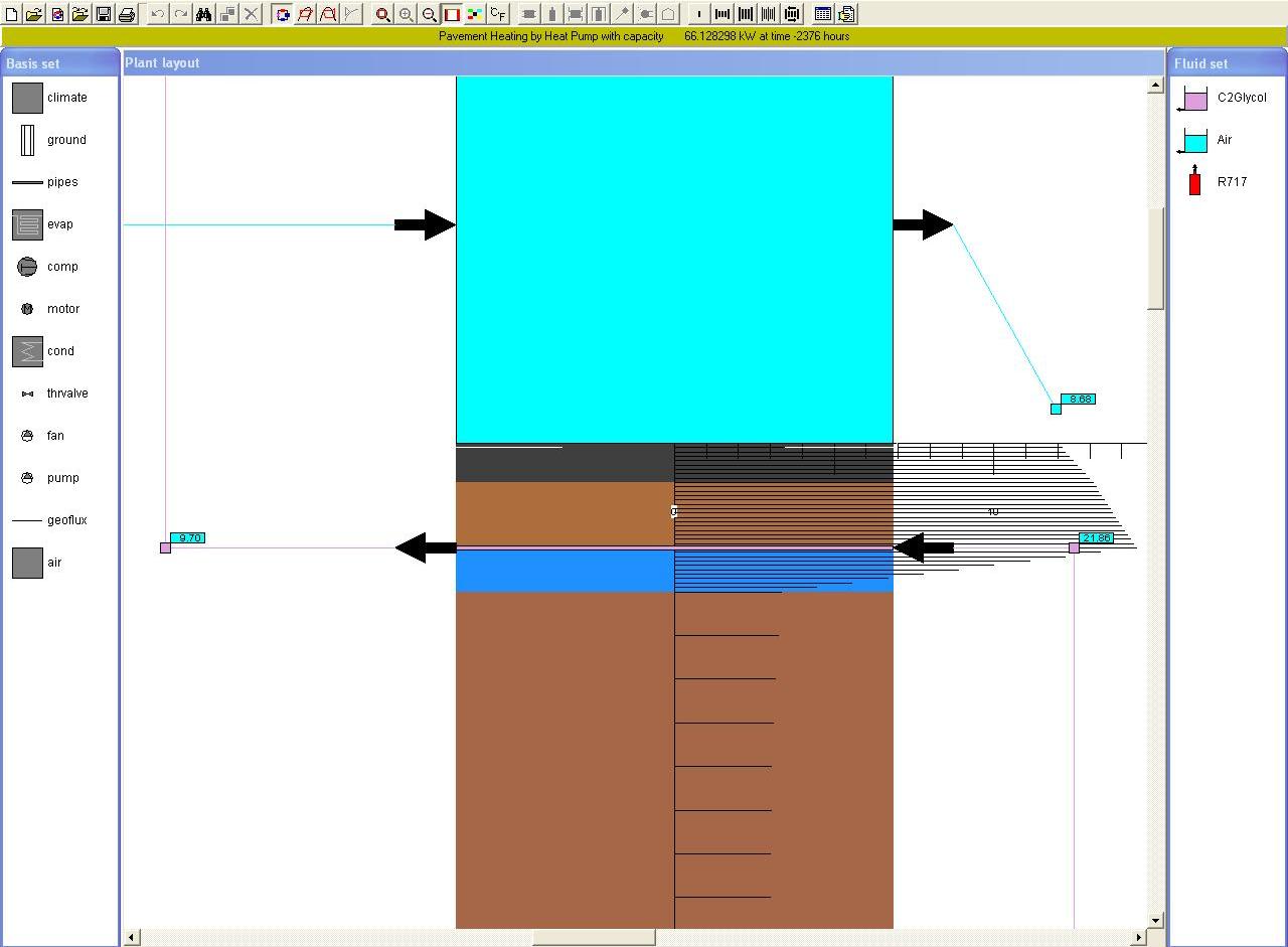
Below is a graph of a detail of a pavement structure with a blue polystyrene insulation between
a gravel and a clay layer.